This new paper in the JEP explains how to run a much better version of the bootstrap. Some of you have heard about this from me before, but many probably have not. I’m passing it on as a public service announcement.
The conventional bootstrap randomly draws observations/clusters, with replacement, from the original sample. This has the problem that if you have a bunch of FEs in your regression (and who doesn’t?) you can get a draw of the data where the FEs perfectly predict treatment status. In that case the bootstrap replicate will fail, causing the dreaded red “x” in your Stata output.
But there is a simple and elegant solution to this. What the bootstrap effectively does is reweight the original sample. In any given draw, some observations get a higher weight (because they are selected more) and some get a lower weight (because they are selected less). What this means is that you can instead run the bootstrap by randomly assigning continuous weights, and bounding them to be above zero:
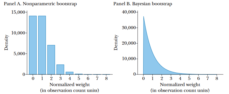
This “Bayesian bootstrap” avoids the collinearity problem from the conventional bootstrap (which Andrews et al. call the “nonparametric bootstrap”), since no observation ever gets a weight of zero.
Read the whole paper to see more about why this approach is better. Or you can just trust me, and switch to this approach that will play much nicer with your fixed effects.